Texture Image Extrapolation for Compression
Sung-Won Yoon and Seong Taek Chung
EE368B, Stanford University
I. Introduction
II. Non-parametric Sampling
III. Estimation Using Subband Decomposition of Wavelet
Coefficients
IV. Estimation by Induced Correlation
V. Conclusions
I. Introduction
Image compression can be achieved if we can recover the whole image from
partial descriptions of the image. With only a fraction of the original
information, the decoder can reconstruct the original image from this fractional
information. Our expectation is that the reconstruction of
the original image can be achieved with small loss by exploiting the inherent
property of the original image. We approach this problem with three
different methods - non-parametric sampling, estimation using subband decomposition
of wavelet coefficients, and estimation by induced correlation. As
a starting point, we will be using texture images because of its abundance
in repetitive information that is more feasible for utilization.
II. Non-parametric Sampling by Pattern Matching
1. Motivation
We want to transmit as small amount of data as possible without worsening
the quality of image significantly. In this section, as one of approach,
we consider the case where texture with a hole is transmitted and a hole
is filled up by pattern matching at the receiver. In fact this has been
investigated in other literatures [1][2],
but we extend this concept more here. What we do here is that we reconstruct
the empty area by comparing the window around one pixel with other non-empty
area. For example, in the figure below, we want to fill the red pixel.
To find the value corresponding to this red pixel, we make a dotted red
box and then do full search over the whole image to find the best matching
blue dotted box.
Our target is to fill the empty area so that the resulting
image approaches the original image.

2. Texture with a Big Chunk of Hole
First, we consider the case where a big hole exists in the texture. This
hole is filled by pattern matching assuming Markov model on texture. Markov
model assumption decides the size of the window. We just provide the result
below. The result is different according to the size of window and the
filling order. But generally, the reconstruction is too sensitive to the
size of window, and the reconstructing time is too long. Good performance
is shown when window size and the filling rotation is adequately chosen.
But here we just show the bad results to emphasize the disadvantage of
this method.
 |
 |
 |
|
original image
|
image with half of its area as a hole |
image reconstructed with 3 by 3 window
|
<Fig.1>Texture with Big Chunk of Hole
3. Texture with Scattered Holes across the Image
Now, we consider the case where many holes are scattered across the image.
As an extreme case we consider the case where only pixels with even row
and even column are retained. (In other words, sub-sampled image is used.).
We assume a known patch of the whole or part of the basic pattern in the
texture. Estimation is done for every 'empty' pixel by block matching
the valid pixels in the given image with the patch. Newly estimated
pixels are incorporated into the estimation as the process goes on.
Next figure shows the extrapolated image with a sufficiently large patch
to cover the basic feature of the texture and the image where the patch
does not fully cover the basic feature. In both cases, satisfactory
extrapolation is achieved with one fourth the information of the original
plus the small patch infomation which becomes negligible as the image gets
larger. Note that in both cases, erroneous or minute deviation from
the general feature of the pattern is lost or altered in the estimated
images.
 |
 |
| Original Image |
Extrapolated Image (patch hold the whole feature) : 23.1338 dB |
 |
 |
 |
| Original Image |
Patch used |
Extrapolated Image : 20.8683 dB |
<Fig.2> Evenly Spaced Texture Filling
4. Conclusion
For the first method, performance is good when the window size and
the reference is chosen cleverly, but the reconstruction time is generally
long and the performance is not guaranteed for general sets of images.
For the subsampled case, even with a patch that does not hold the whole
feature of the texture, it works well. The content of the feature
in the patch is also the major factor in the performance.
III. Estimation Using Subband Decomposition of Wavelet
Coefficients
1. Motivation
By use of subband decomposition of an image, any given image can be decomposed
into 'bandpassed' images. In the Laplacian pyramid structure[3],
as used in the predictive coding, original image is decomposed into approximate
octave-width subband images. In the wavelet transform decomposition, the
original image is decomposed into oriented spatial frequency bands (horizontal,
vertical, and diagonal), which we will refer to as details. In Fig.3,
by exploting the correlation between C and B, we want to estimate the components
in A.
Our target is to explore into using these decomposed subband
images or transform coefficients to estimate unknown subband components.
 |
|
<Fig.3> Ocatve-width Band Splitting
|
2. Model
Our model of the decomposition assumes the existence of spatial locality
and self-similarity between subbands. Fig.4 and Fig.5 show the similar
features within the subbands as images (or coefficient). These features
are mainly the edges in the image, and they clearly show self-similarity
and locality, only different in the scaling. By exploring these inherent
similarities between subbands, we try to find a linear relation (we will
explain this relation later) to estimate new subband pixels or coefficients.
Under the assumption of the propagation of mapping relations between two
adjacent subbands to a different pair of adjacent subbands, mapping found
in one pair is used in the mapping of another.
 |
 |
 |
|
L2 plane
|
L1 plane |
L0 plane
|
<Fig.4> Laplacian Subband Images ("checkerboard", 3 level, gaussian
3X3 filter)
 |
 |
 |
|
Detail 3
|
Detail 2
|
Detail 1
|
<Fig.5 > Wavelet Transform Coefficients ("checkerboard",
diagonal details, 3 level decomposition, bior 2.2 filter)
When using the Laplacian pyramid structure or the wavelet decomposition,
there is a decrease in the size of the plane(image) from subband to subband.
For example, if the lowest Laplacian plane, L0, is of size N by N, then
the next plane L1 is of size N/2 by N/2. Therefore, if we can estimate
the L0 from a lowpass filtered image of size N/2 by N/2, we can achieve
compression by transmitting only the N/2 by N/2 image and estimating the
high frequency subband at the decoder.
Because there is a reduction of four to one from (higher frequency)
subband to (next-lower frequency) subband, the reverse process of estimation
involves one-to-many mapping[4]. Estimating from the
(lower frequency) subband to (next-higher) subband requires each pixel
in the lower subband (we will refer these pixels as the parent pixels)
to predict 4 pixels in the higher subband (we will refer these pixels as
the children pixels). Therefore, our model has each parent pixel associated
with four functions that map the intensity value of the parent pixel to
each of the children pixels, respectively. It is in finding these functions
that define our 'relations' among subbands. Under the assumption of self-similarity
of the pixels among subbands, the four functions were simplified in our
model to scaling functions of the parent pixel value. In other words, the
children pixel values are described by the pixel value of its parent times
a scalar that characterizes the mapping from the parent to each child.
The visual explanation of this paragraph is given in the next figure.
 |
|
<Fig.6> One to Four Mapping between Subbands
|
3. Methodology
A. Laplacian Image Or Wavelet Coefficients
From the visual inspection of the three Laplacian plane images, there exists
a strong similarity in the 3 images, differing only in spatial scale. This
was the motivation behind the investigation of an image-based method in
estimating the highest frequency plane.
On the other hand, wavelet transform coefficients are characterized
by their similarity and locality we assumed in our model and thus fit perfectly
as our source of experimentation. To have a better understanding of the
structure of the wavelet transform coefficients and the inherent spatial
similarities, experiment started with a simple synthetic image - checkerboard.
This image has ideal horizontal, vertical, and diagonal structure. When
a 3 level wavelet transform was used with biorthogonal filter of length
2.2, the resulting coefficients present a very simple structure and similarity.
Unlike the Laplacian images, the wavelet coefficients had a large different
in the range of values from plane to plane. Normalization was necessary
to correctly determine the scalar function mapping of each parent pixel
to its children pixels. It was also needed for comparison of blocks in
adjacent planes of the decomposition.
B. Procedure
Our experiment was done with texture images because of the abundance in
the repetitive structure within the image that can be exploited in hopes
of finding a good estimation mapping. The general process goes as
follows.
| 1) decompose input image - 3 levels (A, B, C) |
2) normalize  and
and  by
normalizing factor by
normalizing factor to get
  and
and  |
3) find the mapping from pixels in C to B
. |
4) find the best match in the minimum MSE or maximum correlation
sense best matching pixel coordinate
.
or
. |
| 5) if multiple best matches, find the one closest in Euclidean distance
to the parent pixel |
6) estimate the 4 children pixel of the current pixel in B
. |
C. Search Regions
Full area search was conducted to make more use of the repetitive structures
in texture images.
3. Results
A. Laplacian Images
In contrast to the apparent locality of features in the 3 subband images,
there was a lack of similarity among subbands. As mentioned, the dominant
features of the subband images are the edges which represent transition
of pixel values. Inspecting a one dimensional slice, of a sharp edge, as
shown in the Fig.7, there is a large difference in the slopes of the edge
between subbands (Note also that the pixel ranges are doubled going from
L2 to L1 and L1 to L0). L2 plane shows a gradual transition of the edge
over a number of pixels, L1 plane shows a sharper transition, and L0 plane
shows the sharpest transition existing over a small interval. This phenomenon
can be explained by the frequency components each subband contains. Since
the L2 plane contains the lowest frequency components of the three Laplacian
planes, the lack of high frequency components result in the gradual transition.
On the other hand, L0 plane contains the highest frequency components,
and that explains the sharp transition describing an edge. Such an analysis
can be extended in 2 dimension such as the subband images. Therefore, our
assumption of similarity among subbands breaks down in the Laplacian image
based approach, and a simple implementation of our proposed algorithm fails.
 |
 |
 |
|
Slice in L2 Plane
|
Slice in L1 Plane
|
Slice in L0 Plane
|
<Fig.7> Slices in the Laplacian Image Planes
B. Wavelet Coefficients
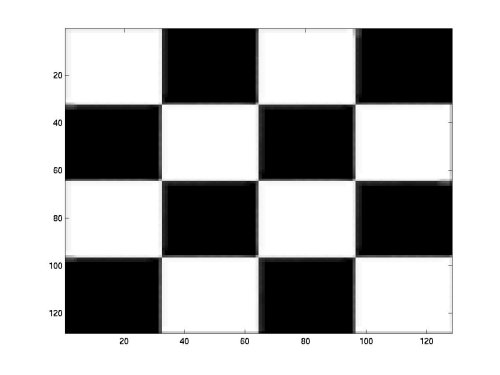
As shown in Fig.8, the wavelet coefficients of the ideal checkerboard image
clearly show locality and similarities between different subbands. The
proposed method works fairly well with this particular image although it
has artifacts at the edges. These artifacts are mainly caused by the inaccurate
magnitudes of the estimated pixel values after the normalization of the
planes for processing. Fig.9 show the resulting reconstructed image
with the estimation (using minimum MSE or maximum correlation criteria)
with the PSNR, respectively. Since there was a limited number
of values for an ideal checkerboard image, Gaussian noise was added to
the ideal image and the same process was carried out. The resulting
image had degradation compared to the ideal image, a drop of 5 to 6 dB
in PSNR.
 |
 |
 |
|
Vertical Detail 3
|
Vertical Detail 2
|
Vertical Detail 1
|
<Fig.8> Vertical Detail Coefficients of Wavelet Transform (bior
2.2)
 |
 |
| Estimated Image (MMSE) : 24.3735 dB |
Estimated Image (Correlation) : 23.7204 dB |
<Fig.9> Estimated Images of Ideal Checkerboard
Statistical characteristics of the coefficient values in each subband
plane shows increase in the variance and range of values from the highest
frequency subband(D1) to the lowest one(D3). The range of the value
increases because the D3 planes are formed after filtering 3 times as compared
to a single filtering for the D1 planes. Since the wavelet transform is
a filtering process, the coefficients are determined by the filter taps
and neighboring pixels that are input to the filter. For this reason, ranges
varied for different images and for different filters. This range difference
between subbands was the major cause of error and difficulty. As mentioned,
normalization was necessary to compare blocks in D2 and D3. It was also
needed to determine the scalar factors in the parent to children mapping.
Although efforts were made on figuring out the range differences, there
was no general trend. Normalization by the dynamic range of coefficient
pixels or the variance of the pixels in each plane were attempted, it did
not improve the results when real texture images were used. Another
major problem was the near zero mean and the difference in variance from
plane to plane. Near zero values of the parent pixels were set to
zero and consequently they were non-significant coefficients. If
near zero values were used in mapping and estimation, they resulted in
erroneous large scaling coefficients, so they need to be set to zero.
Since the mean values of each plane was near zero and the variance decreased
from D3 to D1, many valid mappings in D3-D2 pair were not being fully utilized
in D2-D1 pair mapping due to the thresholding process described.
An appropriate tradeoff point was not available from experimentations.
The assumption of mapping propagation from one adjacent subband pair
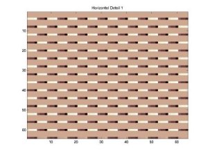
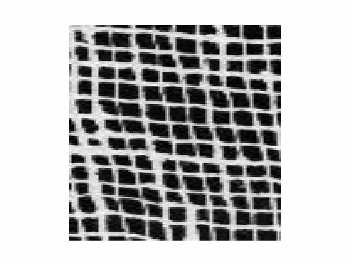
to another does not generally hold for texture images. Figure shows the
horizontal detail planes (D1, D2, and D3) for a real texture image and
an ideal dense checkerboard pattern image. From the visualization of the
texture image coefficients, structure is very difficult to find in the
D3 plane. There is an increase in structure in D2 and D3 planes.
Thus, trying to find a mapping in the more unstructured coefficients to
estimate more structured coefficient mapping results in a random like behavior
of the estimation. Even with the same checkerboard pattern differing
only in the density of the patterns in the image, there is a noticeable
difference in the wavelet coefficient decomposition. Specifically, due
to lack of similarity in D3 and D2, the mapping of D3 to D2 would not be
the same as from D2 to D1. Therefore, a mapping acquired from D2
and D3 does not generally provide a correct mapping of the coefficients
from D2 to D1 which is our source of estimation.
 |
 |
 |
|
Horizontal Detail3 (Texture)
|
Horizontal Detail 2 (Texture)
|
Horizontal Detail 3 (Texture)
|
 |
 |
 |
|
Horizontal Detail 3 (Checkerboard)
|
Horizontal Detail 2 (Checkerboard)
|
Horizontal Detail 1 (Checkerboard)
|
<Fig.10> Vertical Detail Coefficients of Wavelet Transform (bior
2.2)
4. Conclusion
Although there are visual similarities in the Laplacian image or the wavelet
coefficients of subband decomposed image, the exploitation of those characteristics
was not as obvious. An appropriate model plays a major role in understanding
the problem of one to four mapping between subbands under the assumption
of similarity and locality. With our simplified model, image-based
approach to finding the mapping similarities among subband images was not
feasible due to the characteristics of the bandpassed signals in spatial
domain. With the wavelet coefficients, similarity and locality fit
into our model and we were able to get some results for a simple and ideal
image. But as we implemented on real texture images and different
images, the estimation process was not satisfactory. There are many
complications involved that make the estimation process not a simple one.
The statistical characteristics of the coefficient values from one subband
to another differs depending on the image as described in the results.
These difference hinder a good comparison of the block matching and the
the properly ranged estimation of the estimated coefficients. The
assumption of propagation of mapping relations among two different pairs
of subbands does not hold in general. Therefore, the mapping from
D3 to D2 does not necessarily estimate the coefficient values of D1 from
D2. This suggests a possible approach of determining the confined
mapping from D2 to D1 in the statistical workframe. Due to limit of time
allotted for this project, we did not have the chance to pursue any further
into this matter.
IV. Estimation by Induced Correlation
1. Motivation
What we tried in the previous section was to utilize the statistical correlation
between each plane (image or wavelet coefficients). The previous results
show that our approach doesn't yield satisfactory results. The main reason
is due to the fact that even though we know the rough relation between
upper plane and lower plane, the ignorance of exact statistical relation
prevents us from approaching this problem effectively.
To solve this problem we have to understand the statistical relation
of pixels between each plane. But to measure the statistical property of
each image is a hard job. Especially looking for the statistical relation
between wavelet transform coefficients requires a lot of computation.
Here we approach this basic problem with a new paradigm. Our basic problem
is to reconstruct the original image well by transmitting only a fraction
of the original image. So, rather than just using the planes provided by
wavelet transform (or subsampling) with unknown statistics, we construct
a new transformation in order to construct the set of layer where we can
control the statistical relation between layers completely.
2. Procedures
We only consider the case where two planes exist. Upper plane (the pixel
of which is represented as u) and lower layer (the pixel of which
is represented as l ) is constructed. The system model is given
as below.

The original block of image is given as vector x. u means
the element of upper layer which is not transmitted while l means
the element of lower layer which is transmitted. So here only the ratio
of |l| (the length of vector l) over |y| (the length
of vector y) is transmitted. Even though for notation's convenience
we denote upper plane and lower plane, now these terms have no relationship
with a real upper frequency and a real lower frequency. These planes are
simply the ones constructed to our purpose, so relationship with physical
frequency or space.
Our target in this system is to find the filter B
which maximizes the PSNR at the end of receiver.
| 1. Eliminate the correlation between each component completely using
KLT.
This step is necessary to make the correlation between each component
under our control completely later by correlation filter, B. KLT
means xKLT= A x , where A is the Hermitian of
the eigenmatrix of the original image.
|
| 2. Put xKLT into an invertible filter B such
that the correlation matrix of y ( =B xKLT ) has a "good"
property.
Filter B should be invertible so the estimated image can be reconstructed
later.
"Good" property means that the PSNR is maximized after estimating the
original image using the "layer".
|
| 3. Choose l from y and transmit only l.
y=[y1, ..., yn, ..., ym]
(
=B xKLT ) and our definition of layers are u=[y1,...,
yn], l=[yn+1,..., ym].
So only (m-n)/m of the original image is transmitted.
|
| 4. Estimate u using l.
In order to maximize SNR, the mean square error between estimated
u and real u should be minimized. From linear estimation theory
that filter C=E[ulH](E[llH])-1
minimizes the mean square error. Then mean square error is tr(E[uuH]-E[ulH](E[llH])-1
E[luH]). So we have to find the matrix filter B so
that tr(E[uuH])/tr(E[uuH]-E[ulH](E[llH])-1
E[luH]) is maximized.

|
| 5. Reconstruct xKLT using estimated y. |
| 6. Reconstruct x. |
So the next job is to find the filter B which maximizes the PSNR
at the end of receiver.
3. Design of filter B
| The estimation error for u is
 . .
So noise term at PSNR is the trace of the following matrix.

|
To find the invertible matrix B to minimize the noise is very
difficult job. So we could not solve this for general cases. Even though
we could not solve this problem, this is very interesting problem since
it will guide the systematic approach to construct the planes to reconstruct
the original image by containing of a fraction of the image.
But for the case when n=1 and m=2, we could solve this
problem.
Now the best approach we can do is to find the best-possible sub-optimal
invertible solution. We found the two B below using our test images.
More B could be tested, but this 2 matrixes indeed shows the general
trend quite well.
| General B |
Special B |
One of the easiest solution is to set  when e is not 0.
Then we can estimate u from l by multiplying l by
 . .
And the corresponding noise term in PSNR is  . .
Experimentally we know that the energy concentration property of KLT
is very good. (Indeed in terms of energy concentration property, KLT is
the optimal of all the other transforms.). So even for different images,
the noise term takes relatively stable value. |
For specific images we searched a good matrix filter B. Below
is the filter B, which was designed for the first image in Section
4. Here we call this filter as a special filter.

|
4. Results
In this section as a comparison we compare the estimated image with the
image reconstructed by interpolation of sub-sampled (only odd columns are
taken) image. This is a fair comparison since both of them transmit only
half of the original pixels.
 |
 |
 |
 |
| Original Image |
Extrapolated Image with general B : 17.18 dB |
Extrapolated Image with special B : 19.8187dB |
Interpolated Image : 20.9868dB |
<Fig.12> Estimated Images 1
In preserving the details of textures, this extrapolation method works
much better than interpolation, but in preserving the intensity of the
general shape, interpolation works better. By designing a special filter,
B, the performance gets better. As we explained above, by spending more
time in looking for the best filter B, the performance could improve.
 |
 |
 |
 |
| Original Image |
Extrapolated Image with general B : 15.3313 dB |
Extrapolated Image with special B : 14.7275dB |
Interpolated Image : 12.7236dB |
<Fig.13> Estimated Images 2
In this case, generally extrapolation cases work better than interpolation.
That is because this image has a lot of high frequency component, so interpolation
loses a lot of original image property. On the other hand, extrapolated
image loses the property of original image rather equally through the whole
images, so the degradation is spreaded over all frequencies. What is also
notable is that in case of special filter, here this performs worse than
general filter since the special filter was designed for the first texture
above.
 |
 |
 |
 |
| Original Image |
Extrapolated Image with general B : 29.2755 dB |
Extrapolated Image with special B : 32.2265 dB |
Interpolated Image : 33.6150 dB |
<Fig.14> Estimated Images 3
From here we can see that this extrapolation method work for general
images also. In case of interpolation, the high frequency component of
image is lost, but in case of extrapolation, the jaggy effect appears on
the edges. So it is hard to say what is better than the other.
5. Conclusion
As we could not consider the general case due to the lack of mathematical
skill, we have to make conclusions based on limited cases. As shown in
Section 4, we can find the generally reasonably working filter
B.
If we do search for each image we could encounter good filter B
we could beat the interpolation, but that filter B strongly depends
on the kind of image. Even though we could not find a good B for
all images, from Section 3, we know that good B which beats interpolated
image exist theoretically.
Considering the small number of data that
B and KLT filter has,
the optimal way to transmit low rate image is to find a good B for
each images, and then transmit only a fraction of image with a good B
and KLT filter. As original image grows bigger, the overload of transmitting
B
and KLT filter becomes negligible.
V. Conclusions
We carried out 3 different approaches to achieve compression for
texture images. The first approach was an experimentation and extension
to the ideas in [1] and [2].
The second approach was an investigation into the utilization of correlation
inherent among subbands, especially by use of wavelet transform coefficients.
Third approach was, to an extent, the reverse idea from the second - we
try to control the correlation among the data.
We found out that for texture images, non-parametric sampling method
proves a good method in its performance of achieving compression.
The drawback is the long computation time involved and the dependency of
the window size in the implementation.
Contrary to the visual similarities of the wavelet coefficients images,
there was lack of information to be can be shared between different pairs
of subbands. As a result, trying to find correlation between the
highest two subbands from lower subbands relations does not yield fruitful
results. A statistical framework in the highest two subbands would
be the natural step in further investigating into this approach.
Decorrelating the image pixels by KLT and inducing controlled correlation
is a novel idea that proved to have benefits as well as pitfalls.
Though there were limitations due to lack of mathematical tool to find
and elegant analytical form, this approach is also open to more investigation.
References:
[1] Alexei A. Efros and Thomas K. Leung. Texture
Synthesis by Non-parametric Sampling. IEEE International Conference
on Computer Vision, September 1999.
[2] Li-Yi Wei and Marc Levoy. Fast Texture
Synthesis using Tree-structured Vector Quantization. Proceedings
of SIGGRAPH, 2000
[3] Peter J. Burt and Edward H. Adelson. The
Laplacian Pyramid as a Compact Image Code. IEEE Transaction on
Communications, April 1983.
[4] Alex Pentland and Bradley Horowitz. A Practical
Approach to Fractal-based Image Compression. IEEE Data Compression
Conference, April 1991
Appendix:
Section II: Seong Taek Chung
Section III: Sung-Won Yoon
Section IV: Sung-Won Yoon & Seong Taek Chung


