


EE 368 Final Project
December 1, 2000
Prashant Ramanathan
Overview
Multiple-hypothesis motion-compensated prediction has been used successfully in video compression. In this project, we investigate whether similar techiques yield positive results for disparity-compensated light field compression.
Table of Contents
1. Introduction
2. Background
3. Proposed Method
4. Experiments
5. Results and Discussion
6. Conclusions and Future Work
7. References
8. Source Code
1. Introduction
Image-based rendering is emerging as an important new alternative to traditional image synthesis techniques in computer graphics that rely on geometric, lighting and shading models. Light field rendering [1] [2] is one such image-based technique that, while providing photo-realistic quality, allows the user to freely choose viewing position and direction. In light-field rendering, a set of acquired images are sampled in order to create novel views, and no additional information about the scene is required. The light field data set consists of a collection of images, called light field images. These images are layed out in as 2-D array, resulting in a 4-D data set. An example of such a light field is shown in Figure 1. Equivalently, light fields can be thought of as describing the radiance function in a scene for any arbitrary position and direction. This 5-D function reduces, in free space, to a 4-D function.
|
|
|
|
|
|
|
|
|
|
|
|
|
|
|
|
|
|
|
|
Figure 1: The Flieger light field
The acquisition of light field images is difficult for real scenes or objects. Moreover, light field data sets tend to be extremely large. A light field of an interesting object such as Michelangelo's statue of Night [3], contains tens of thousands of images, requiring over 90 gigabytes of storage for raw data. Compression is, therefore, a necessity for light fields.
Disparity-compensation [4] is currently one of the most effective techniques used for light field compression. It is analogous to motion-compensated prediction in video compression. In this project, we investigate the use of a new technique, multiple-hypothesis prediction, for disparity-compensation. In the existing disparity compensation scheme, only one disparity value is specified for each block in the image. In this investigation of multiple-hypothesis prediction, up to two disparity values are specified. By examining the rate-distortion behaviour of this scheme to the original scheme, we can determine whether multiple-hypothesis prediction is an idea worth pursuing in disparity-compensated light field compression.
2. Background
2.1 Light Field Compression
The first light field compression algorithm appears in the original light field paper itself [1]. Vector quantization and entropy coding are used to compress the data set. In [4], light fields are coded using video compression techniques, such as the Discrete Cosine Transform and motion-compensation. [4] also describes a disparity-compensation based algorithm; disparity-compensation is a concept analogous to motion-compensation in video compression. Explicit geometry models have also been used for light field compression [5] [6], yielding similar results to the disparity-compensation approach [4].
In this project, we will be working only with disparity-compensation as described in [4]. Disparity, a well-known concept in computer vision, describes the translation of a pixel or object between two neighboring images of the scene. Knowing the disparity for a given pixel allows the prediction of that pixel from the corresponding disparity-compensated pixel in the neighboring image. Since the light field camera geometry is known, the translation of pixels between light field image is constrained along a particular direction, described by the epipolar line. Therefore, one disparity value can describe the shift between two neighboring images. If the two views are related by a horizontal translation, then the corresponding disparity will be along the horizontal direction. Likewise, if the two views are related by a vertical shift, then the corresponding disparity will be in the vertical direction as well.
The scheme described in [4] uses 4 reference images to predict a target image. This arrangement is illustrated in Figure 2, where the target image in the center is surrounded by four reference images, all taken from a regularly spaced grid. For this planar camera geometry, if the spacing between all cameras is the same, then the disparity values between each reference image and the target image will be identical.

Figure 2: Light field camera views with constant spacing
The disparity compensated scheme works as follows. The images are divided into blocks of a given size, such as 4x4 or 16x16. For each such block in the target image, a single disparity value is found, such that the resulting mean-squared error between the predicted target image and the true target image is minimized. The predicted target image is found on a block by block basis. For a given block, a corresponding block is found according to the disparity value in each of the reference images. These reference blocks are then averaged together to form one block in the predicted target image.
This disparity-compensation scheme, however, makes a few assumptions. The first is that the object in the images has an ideal Lambertian surface which appears the same from every direction. Although this is approximately correct for matte surfaces, specular or shiny surface violate this condition. This scheme also assumes that a block in the target image has a corresponding block in all the other reference images. This may not be true for two reasons. First, certain portions of the object may be occluded in some of the reference images. Second, if the block is too large, then the disparity may not be constant over the entire block, which means that there will be no corresponding block in any of the reference images. The final assumption, that the disparities are integer-pixel values, will almost certainly be violated for all light field images. A deviation from these assumptions results in a prediction error residual, which may need to be coded based on the required image quality.
2.2 Multiple-Hypothesis Prediction in Video Compression
One early example of multiple-hypothesis motion compensation is B-Frames in H.263 or MPEG. There are three options for how B-frames can be predicted from their immediately neighboring I or P frames. For a given macroblock, either one forward motion vector can be specified for prediction from the previous frame, or one backward motion vector can be specified for prediction from the next frame, or both forward and backward vectors can be specified and the appropriately compensated blocks are averaged to give the prediction signal. This third option is an example of multiple-hypothesis motion compensation, where two vectors are used for prediction. Both theory [7] and practice [8] suggest that using multiple-hypothesis prediction helps in video coding efficiency.
3. Proposed Method
In [8], the prediction is formed by linearly combining blocks from several of the previous frames in the video sequence. A similar idea can be developed for disparity-compensated light field compression. The compression scheme described in [4] specifies one disparity value for a block; all four reference images are compensated based on this value, and averaged to give the prediction signal. A multiple-hypothesis scheme would specify more than one disparity value, as well as specifying the reference images to use for a disparity value. For instance, if two disparity values are used, then the indices of the respective reference images will also be specified. Although this will increase the amount of side information that needs to be sent, the hope is that the decrease in prediction error and, consequently, the decrease in the number of bits required to code this residual will more than make up for the cost.
4. Experiments
In our experiments, we use two sets of images from the Flieger planar light field shown in Figure 1. The ideal experimental setup would test the compression results using multiple- hypothesis prediction for the entire compression system, including residual encoding and hierarchical disparity-compensation, as described in [4]. Building such a system, however, is out of the scope for a class project, so, instead, the rate-distortion performance for just the disparity-compensated predictor is considered.
To be specific, we have the following arrangement. The two selected
sets of light field images from the Flieger
sequence, denoted flieger1 and flieger2, are shown in
Figures 3 and 4, respectively. Each set contains a target
image that is to be predicted, and four neighboring reference
images, that are assumed to be already known. Since the system that
we are analyzing is the predictor, the input is the target image,
and the output is the predicted image. In this context, the rate of
this system is the number of bits required to describe one or more
disparity values, as well as the corresponding reference image index,
if required. A probability density function is assumed for the
disparity values, which are integer values over a specified range.
The distortion measure used is the mean squared error between the
predicted and target images. To obtain the operational
rate-distortion curves, we use the
Langrangian cost function
![]() .
To get a single point on the R-D curve, we fix the value of
.
To get a single point on the R-D curve, we fix the value of
 , and search over the entire range of
disparity values to minimize the Lagrangian cost function. By
varying , we obtain the entire
curve.
, and search over the entire range of
disparity values to minimize the Lagrangian cost function. By
varying , we obtain the entire
curve.

|
||

|

|

|

|
Figure 3: Light field data set flieger1

|
||

|

|

|

|
Figure 4: Light field data set flieger2
In our experiments, we examine three schemes:
For each light field image set, flieger1 and flieger2, we find the rate-distortion curves for various block sizes. Four different block sizes are used: 4x4, 8x8, 16x16, 32x32.
5. Results and Discussion
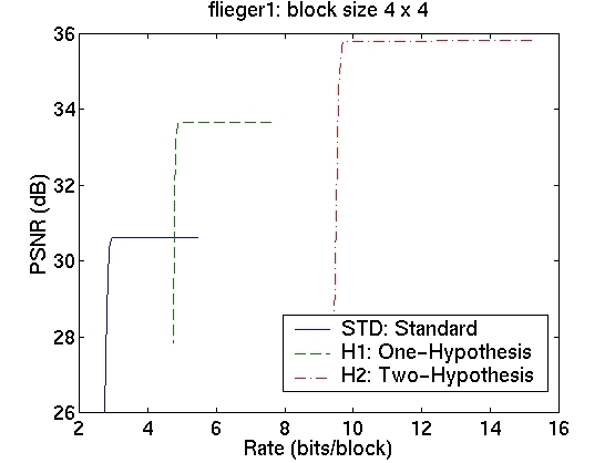
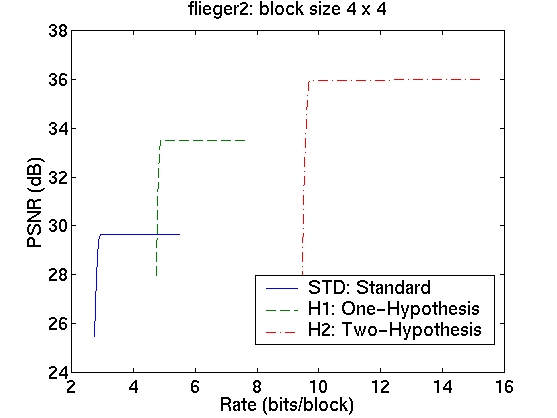
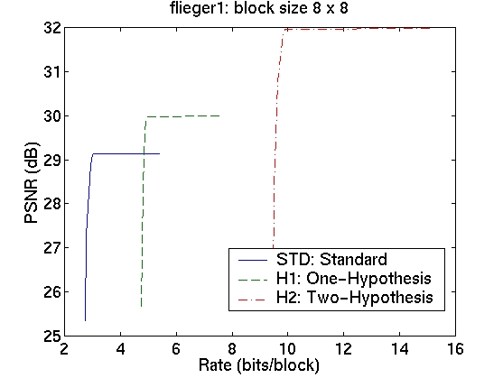
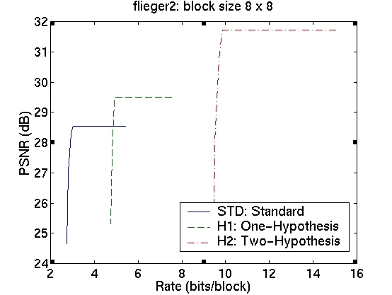
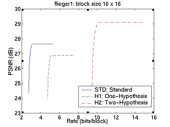
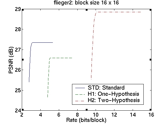
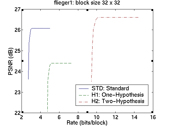
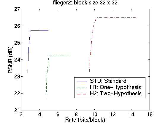
The rate-distortion curves for the three schemes are shown in the table in Figure 5. The curves in the first column correspond to image sequence flieger1 and those in the second column to image sequence flieger2. The rows contain the various block sizes.
|
|
|
|
|
|
|
|
Figure 5: Rate-Distortion curves for flieger1 and flieger2 for varying block sizes
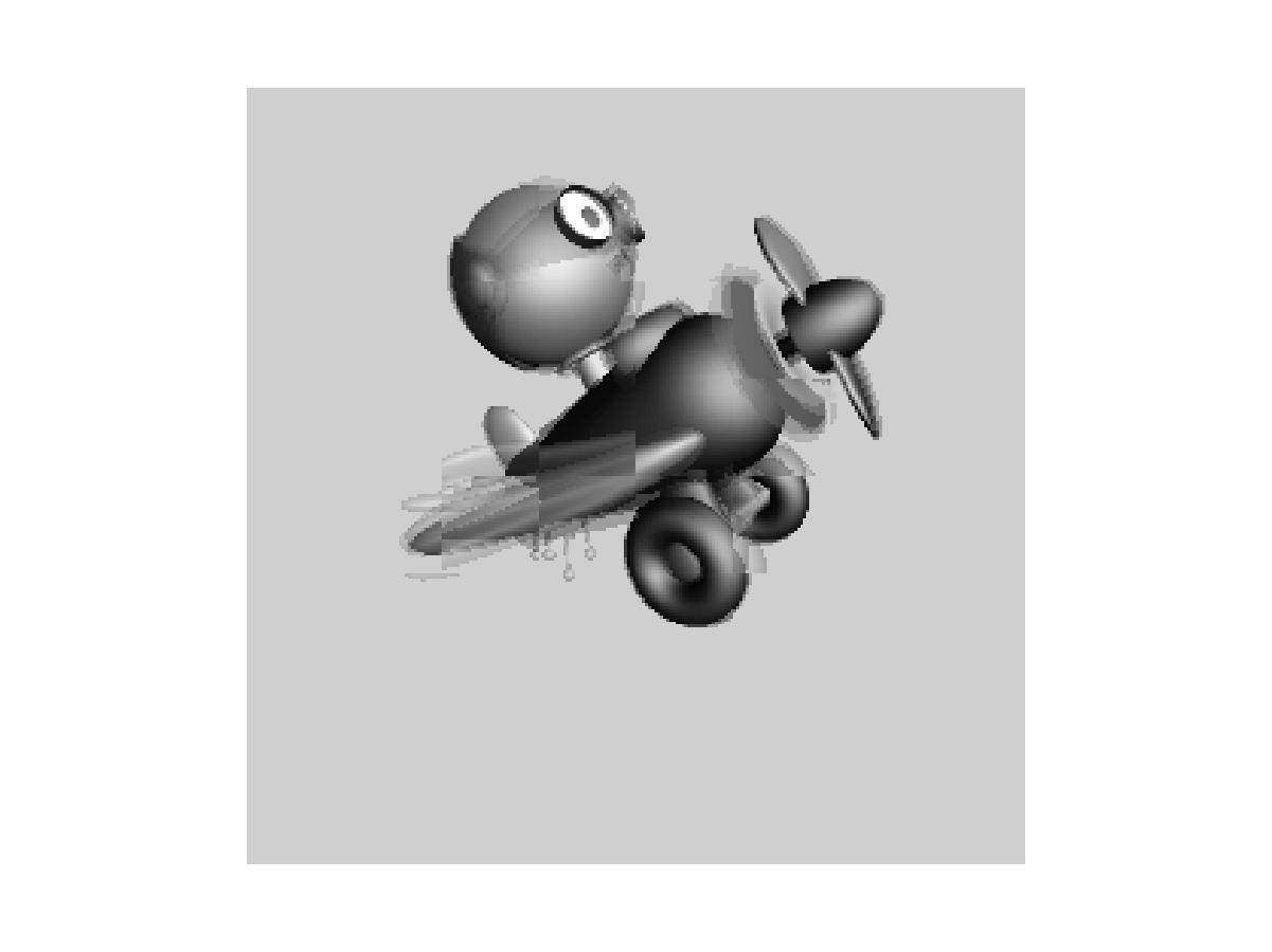
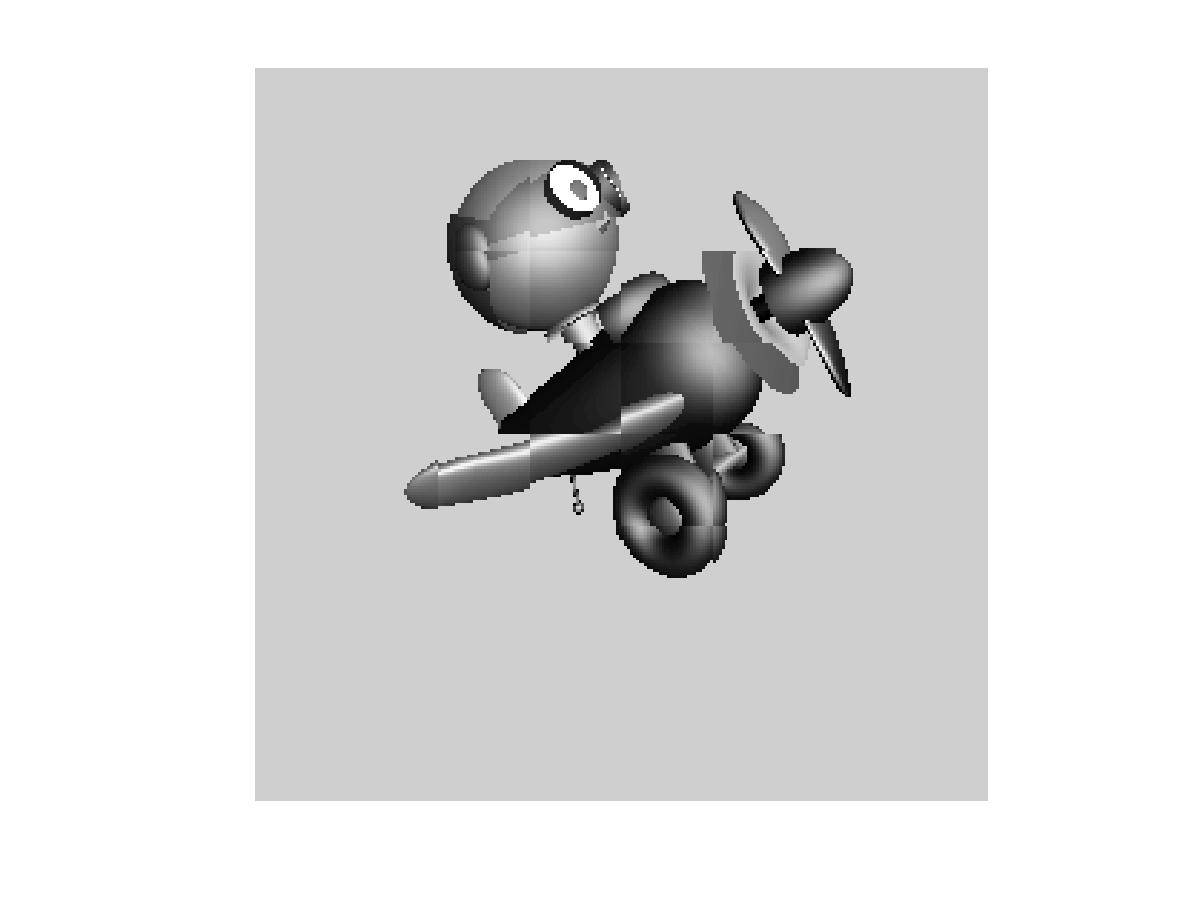
We see that for a block size of 4x4, we obtain a significant improvement in the prediction signal PSNR, when using the two-hypothesis scheme over the standard scheme. For flieger1, this is over 5dB and for flieger2, it is approximately 6.4dB. For this blocksize, the one-hypothesis scheme also performs better than the standard scheme. Figure 6 shows, for the flieger1 sequence, the target image, and the predicted images from all these schemes taken at the "knee" in the R-D curves. We can see that predicted image from the standard scheme is quite smooth relative to the other two images, and that it also contains several ghosting artifacts, especially around the wing. The smoothness is likely a resulting of the averaging of 4 reference images, while the ghosting artifacts are likely due to misalignments of the blocks. The one-hypothesis scheme does a much better job of preserving the edges; however, there are many aliasing artifacts due to the lack of averaging. The two-hypothesis scheme seems to combine the benefits of both; it preserves edges, yet does not show aliasing artifacts.
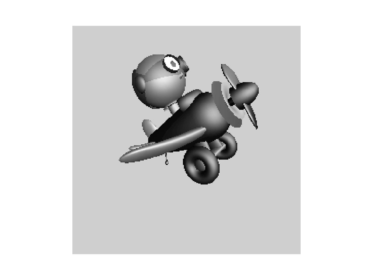
Target Image |

Predicted Image (STD) |

Predicted Image (H1) |
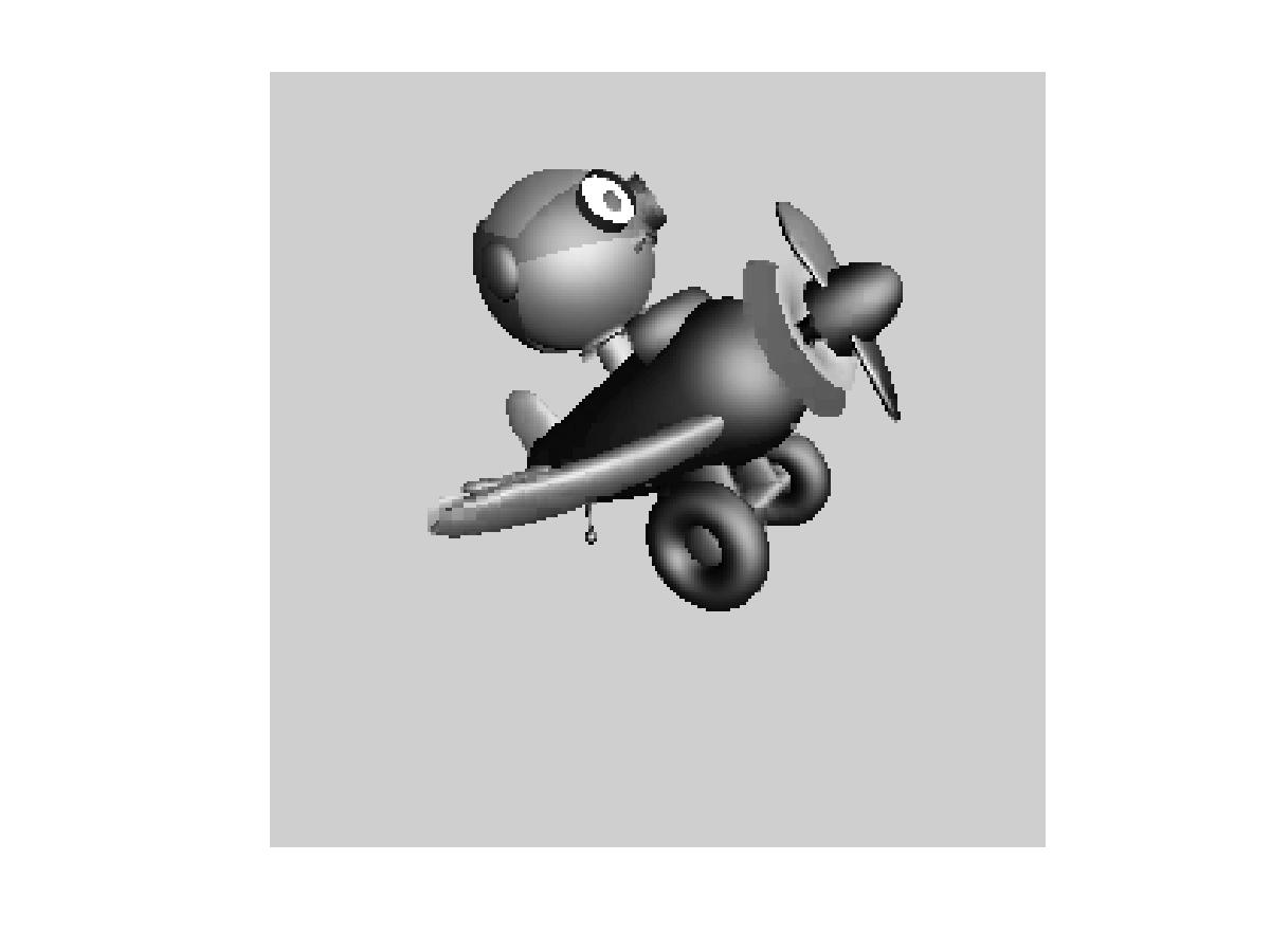
Predicted Image (H2) |
Figure 6: Predicted Images for 4x4 Block Size (flieger1)
As we increase the block size, however, the gains are not as large. With 32x32 blocks, for instance, there is only an improvement of 0.5dB for flieger1 and 0.75dB for flieger2. Also, the one-hypothesis scheme in this case has worse performance than the standard scheme. This is confirmed by examining the images for the flieger1 sequence in Figure 7. The target image, and the predicted images from the three schemes taken at the "knee" in the R-D curves are shown. We see that, as expected, the larger block size leads to worse disparity compensation results for all the schemes. We again see that the standard scheme produces a smoothed image with ghosting artifacts, while the one-hypothesis scheme produces a sharper image, although with significant aliasing. The two-hypothesis scheme attempts to produce a sharp, yet antialiased prediction image.
|
Target Image |
Predicted Image (STD) |
Predicted Image (H1) |
Predicted Image (H2) |
Figure 7: Predicted Images for 32x32 Block Size (flieger1)
We now consider the cost of using the multiple-hypothesis scheme. The standard scheme, operated at the optimal point on the rate-distortion curve, has a rate of approximately 3 bits/block. The one-hypothesis scheme needs to also transmit one of the four reference index, so its rate is 2 bits higher at approximately 5 bits/block. The two-hypothesis scheme needs twice the amount of information, giving it a bit rate of 10 bits/block. The cost of using the superior two-hypothesis scheme comes at a cost of 7 bits; this cost is, however, amortized over all the pixels in a block. This means that the cost per pixel is lower for larger block sizes; however, the gains too are correspondingly lower. Although we observe a decrease in the prediction error, we do not know whether this will translate to an improvement in the performance of the overall system. For conclusive results, we must resort to building and testing the entire system. The fact that we do obtain significant gains in prediction, however, indicates that this might be a worthwhile endeavour.
6. Conclusions and Future Work
In this project, we have demonstrated a multiple-hypothesis scheme for disparity-compensated light field compression. The initial results on a limited set of data indicate that prediction error can be decreased significantly by using such a scheme.
As future work, these experiments should be repeated on several other data sets including, especially, real light field imagery. If results from these experiments confirms the initial findings that significant reduction in prediction error are possible, this scheme should be incorporated into a working light field compression system. In this manner, it can be determined whether the reduction in prediction error translates to an overall compression gain.
7. References
8. Source Code
runTests.m