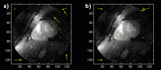
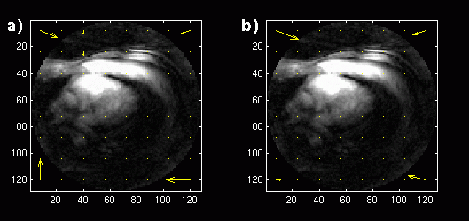
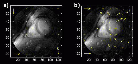
Figure 1. a) Reconstructed image with displacement vectors for each block shown superimposed. Long-term
MCP is used with a buffer of 18 images. b) Reconstructed image with displacement vectors for MCP
with a single image buffer.
Matlab Investigation of Motion-Compensated Prediction with the Cardiac Studies
After the block-matching estimation was written in Matlab, it was tested using some simple image sequences created in Matlab, for example small blocks moving with different periods in different directions. The same sequences were tested with a gradient background. (As an aside, it was interesting to note that when the blocks moved in the direction of the gradient, occlusion of the background caused some errors in the displacement vectors due to a different sum of absolute errors.) Once the function was verified, it was run in Matlab with DCT compression of the error images and uniform quantization of each block of the error images. Rate-distortion curves could not be created in Matlab without Huffman code, and so the lossless part of the compression system was only addressed in the C code. We did obtain very useful information from the spatial displacements, time buffer indices selected, and error images that allowed us to make good guesses of the rate-distortion performance.
Testing MCP with the Original Sequences
All images were of size 128 by 128.
The block matching function used a block size of 16 by 16 pels, meaning it returned
a total of 64 displacement vectors for dx and dy.
To find the displacement vectors, each buffered block was shifted 16
times along the horizontal and vertical
axes (in other words, each block was shifted 8 pixels
in each of 4 directions) for each of the buffered previously reconstructed
frames. The sum of absolute differences (SAD) was computed for each shift,
and the minumim SAD was used to select each block's values for dx
and dy.
Since a heart cycle of about 16 frames was measured for the sequences,
a buffer of 18 frames was used for long-term
memory prediction of the original two sequences.
The Matlab MCP and reconstruction was first applied to the images in the short-axis study. Since a long-term memory buffer size of 18 was used, the first 19 frames were applied to the algorithm and reconstructed, with the 19th frame constructed with blocks from the entire buffer. This reconstructed image is shown in Figure 1a. Vectors representing the x and y displacement values for each block are shown superimposed on the image at the center of each block location. The same 19 frames were then reconstructed with a buffer size of 1. The reconstructed image and displacement vectors are shown in Figure 1b:

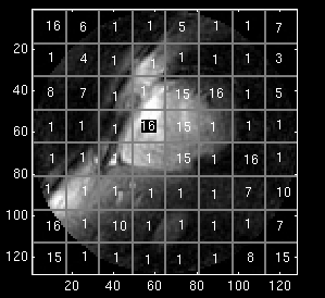
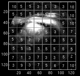
For the long-term memory prediction, we show the reconstructed image with the block edges superimposed and the time buffer indices of each block in Figure 2. Here, 1 corresponds the the index of the previous reconstructed frame, and 18 would correspond the the furthest frame in the time buffer (in this case, the first frame.)
We expect three things of long-term memory MCP and reconstruction with the synthetic sequence:
The time displacement for each block was indeed 5, meaning that the correct quantized image was selected from the frame buffer, verifying our first test condition. The displacement vectors are plotted in Figure 7. Note that now there is a significant difference between vectors using different buffer sizes. For long-term memory MCP, the vectors were zero everywhere, except at the 4 corners outside the image where the displacement selected corresponded to the lowest sum of quantization noise, satisfying our second test condition.
This means that two-thirds of the data used to construct the current image were also used to construct the previous image. This means that subsequent images in the sequence are strongly correlated, and it is reasonable to expect that long-term memory prediction will often select the previous reconstructed frame.
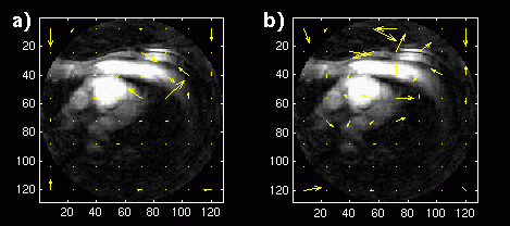
We tested this by removing frame-to-frame data dependencies. We applied motion-compensated prediction and reconstruction to temporally sub-sampled versions of the image sequences. We started by sub-sampling both by a factor of six. The displacement vectors for the reconstructed frame using a single image and a long-term buffer are shown in figures 9 and 10. Now that each frame comes from a completely different data set, the single-frame prediction does much worse compared to when a long-term buffer is used.
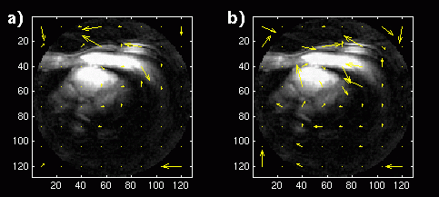
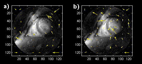
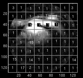
Figure 11 shows the values of the time buffer indices (equivalent to time displacement) for each block in each of the two predicted images. Now that the two image sequences are uncorrelated from frame to frame, very few of the blocks select the previous reconstructed frame.
 b)
b)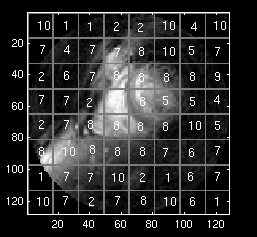
An image sequence with a frame rate of 3 frames per second is not acceptable for a cardiac sequence. However, an image sequence with a frame rate of 9 frames per second might be acceptable. We sub-sampled the original 18 fps image sequences by a factor of two. The displacement vectors for the coronary image sequence tests are shown in Figure 12. There is still a significant difference in the displacement vectors between the long-term memory and single-frame predictions, because now only one-sixth of the data is the same between subsequent image frames.
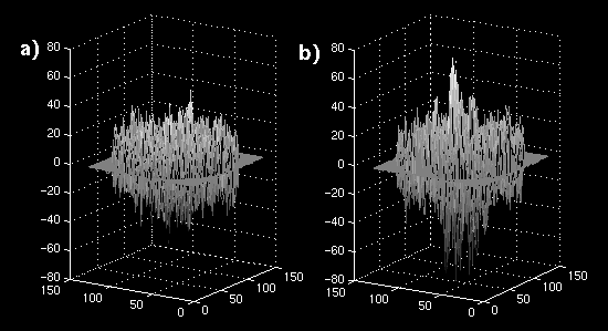
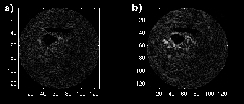
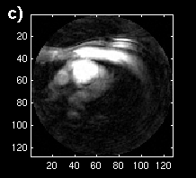
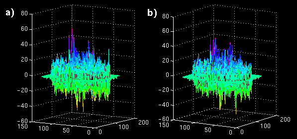
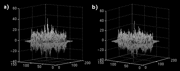
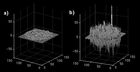
The error images are shown as mesh plots in figure 13 for magnitude comparison. The error is not reduced as significantly as in the synthetic sequence, but there is a distinguishable difference in a region of blocks. The error images are displayed in Figure 14 (a and b) to the same windowed levels. A reference image is shown in Figure 14c to gauge the locations of highest error in the single-frame MCP. Note that the error peaks are located in the region of highest heart motion, meaning that long-term MCP is picking a frame for those blocks closer to the same position in the cardiac cycle.
